3. Classification
Motivation
To get small handful possible number of outputs instead of infinite number of outputs
Logistic regression (Classification)
Output is either 0 or 1
Sigmoid function
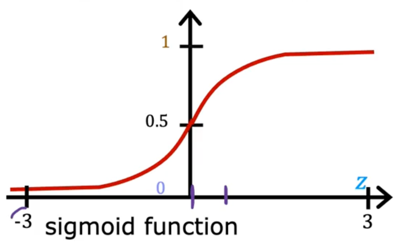
outputs value between 0 and 1
g(z)=1+e−z1 (0<g(z)<1)
Steps
- define z function
fw,b(x)=z=w⋅x+b
- take z function to sigmoid function
g(z)=1+e−z1
Logistic regression
→ fw,b(x)=g(w⋅x+b)=1+e(w⋅x+b)1=P(y=1∣x;w,b)
The probability that class is 1
- example
- x is tumor size
- y is 0(not malignant) or 1(malignant)
- f(x) = 0.7 → 70% chance that y is 1
- P(y=0)+P(y=1)=1
- fw,b(x)=P(y=1∣x;w,b)
- probability that y is 1, given input x, parameters w,b
Decision boundary
Prediction: y^
Is fw,b(x) ≥ 0.5?
- Yes: y^=1
- No: y^=0
When is fw,b(x) ≥ 0.5?
- g(z) ≥ 0.5
- z ≥ 0
- w⋅x+b ≥ 0 → predicts 1 (when w⋅x+b < 0 → predicts 0)
Cost Function
Squared error cost
J(w,b)=m1∑i=1m21(fw,b(x(i))−y(i))2
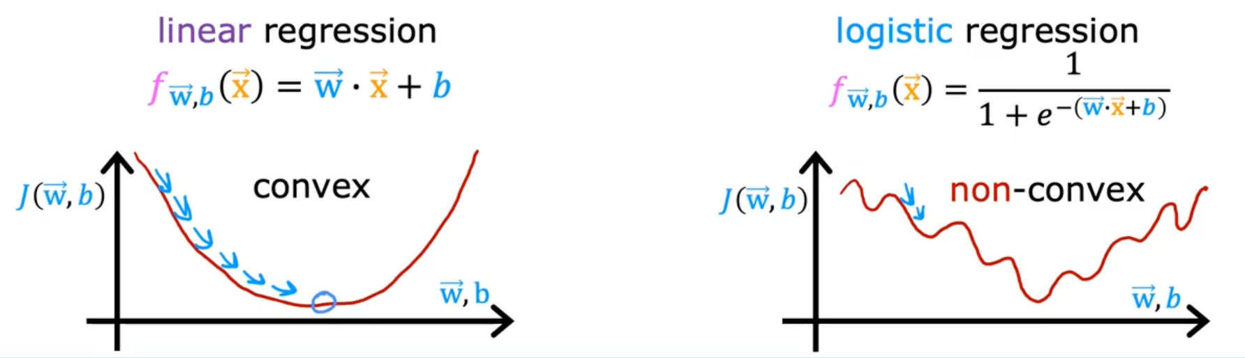
Squared error cost is not a good choice for logistic regression because it can have multiple local minima
21(fw,b(x(i))−y(i))2
- → Loss function L(fw,b(x(i)),y(i)))
Logistic loss function
L(fw,b(x(i)),y(i)))
- −log(fw,b(x(i))) if y(i)=1
- −log(1−fw,b(x(i))) if y(i)=0
When loss close to 0, the predictions is close to the answer
Cost
Loss function will make a convex shape that can reach a global minimum
J(w,b)=m1∑i=1mL(fw,b(x(i)),y(i)))
- −log(fw,b(x(i))) if y(i)=1
- −log(1−fw,b(x(i))) if y(i)=0
Simplified Cost Function
L(fw,b(x(i)),y(i)))=−y(i)log(fw,b(x(i)))−(1−y(i))log(1−fw,b(x(i)))
- if y(i)=1
- L(fw,b(x(i)),y(i)))=−1log(fw,b(x(i)))
- if y(i)=0
- L(fw,b(x(i)),y(i)))=−1log(1−fw,b(x(i)))
Loss function
L(fw,b(x(i)),y(i)))=−y(i)log(fw,b(x(i)))−(1−y(i))log(1−fw,b(x(i)))
Cost function
J(w,b)=m1∑i=1m[L(fw,b(x(i)),y(i)))]
- = −m1∑i=1m[y(i)log(fw,b(x(i)))+(1−y(i))log(1−fw,b(x(i)))]
Gradient Descent
J(w,b)=−m1∑i=1m[y(i)log(fw,b(x(i)))+(1−y(i))log(1−fw,b(x(i)))]
repeat {
wj=wj−adwjdJ(w,b)
- dwjdJ(w,b)=m1∑i=1m(fw,b(x(i))−y(i))xj(i)
b=b−adbdJ(w,b)
- dbdJ(w,b)=m1∑i=1m(fw,b(x(i))−y(i))
} simultaneous updates
Gradient descent for logistic regression
repeat {
wj=wj−a[m1∑i=1m(fw,b(x(i))−y(i))xj(i)]
b=b−a[m1∑i=1m(fw,b(x(i))−y(i))]
}
Linear regression model
fw,b(x)=w⋅x+b
Logistic regression
fw,b(x)=1+e−w⋅x+b1
- Same concept
- monitor gradient descent (learning curve)
- vectorized implementation
- Feature scaling
The problem of overfitting
Linear regression
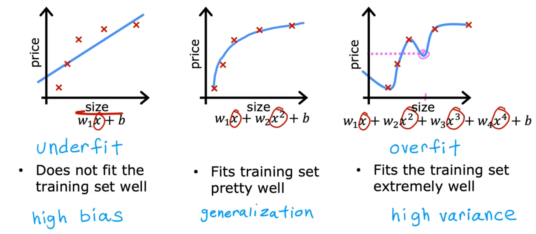
Classification
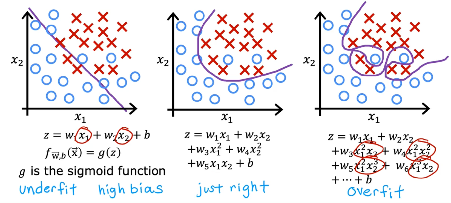
Addressing overfitting
- Collecting more training examples
- Selecting features to include or exclude
- Reduce the size of parameters
Cost Function to Regularization
Intuition
minw,b2m1∑i=1m(fw,b(x(i))−y(i))2
- small values w1, w2,…wn,b → simpler model less likely to overfit
- J(w,b)=2m1∑i=1m(fw,b(x(i))−y(i))2
- Lambda λ
- regularization parameter λ > 0
- J(w,b)=2m1∑i=1m(fw,b(x(i))−y(i))2+2mλ∑j=1mwj2+2mλb2
- mean squared error
- 2m1∑i=1m(fw,b(x(i))−y(i))2
- Regularization term
- 2mλ∑j=1mwj2
- Can include or exclude b
Regularization
minw,bJ(w,b)=minw,b[2m1∑i=1m(fw,b(x(i))−y(i))2+2mλ∑j=1mwj2]
- Linear regression example
fw,b(x)=w1x+w2x2+w3xe+w4xr+b
choose λ=1010 → underfits
choose λ=0 → overfits
Regularized linear regression
minw,bJ(w,b)=minw,b[2m1∑i=1m(fw,b(x(i))−y(i))2+2mλ∑j=1mwj2]
Gradient descent
repeat {
wj=wj−adwdJ(w,b)
b=b−adbdJ(w,b)
}
- wj=wj−adwdJ(w,b)
- =m1∑i=1m(fw,b(x(i))−y(i))xj(i)+mλwj
- b=b−adbdJ(w,b)
- =m1∑i=1m(fw,b(x(i))−y(i))
- don’t have to regularize b
Implement gradient descent with regularized linear regression
repeat {
wj=wj−a[m1∑i=1m(fw,b(x(i))−y(i))xj(i)+mλwj]
b=b−am1∑i=1m(fw,b(x(i))−y(i))
}
wj=wj−a[m1∑i=1m(fw,b(x(i))−y(i))xj(i)+mλwj]
- wj=1wj−amλwj−am1∑i=1m(fw,b(x(i))−y(i))xj(i)
- wj=wj(1−amλ)−am1∑i=1m(fw,b(x(i))−y(i))xj(i)
- usual gradient descent update : am1∑i=1m(fw,b(x(i))−y(i))xj(i)
- shrink w : (1−amλ)
How we get the derivative term
dwjdJ(w,b)=dwjd[2m1∑i=1m(f(x(i)−y(i))+2mλ∑j=1nwj2]
- = 2m1∑i=1m[(w⋅x(i)+b−y(i))2xj(i)]+2mλ2wj
- = m1∑i=1m[(x⋅x(i)+b−y(i))xj(i)]+mλwj
- = m1∑i=1m[(fw,b(x(i))−y(i))xj(i)]+mλwj
Regularized Logistic Regression
Logistic regression
z=w1x1+...+wnxn+b
Sigmoid function
fw,b(x)=1+e−z1
Cost function
J(w,b)=−m1∑i=1m[y(i)log(fw,b(x(i)))+(1−y(i))log(1−fw,b(x(i)))]+2mλ∑j=1nwj2
- minw,bJ(w,b)
Gradient descent
repeat {
wj=wj−a[m1∑i=1m(fw,b(x(i))−y(i))xj(i)]+mλwj
b=b−a[m1∑i=1m(fw,b(x(i))−y(i))]
}