Regression with Multiple Input Variables
Deep dive into multiple linear regression, vectorization, gradient descent, feature scaling, and polynomial regression.
10 min read
• Updated: March 20, 2024 2. Regression with multiple input variables
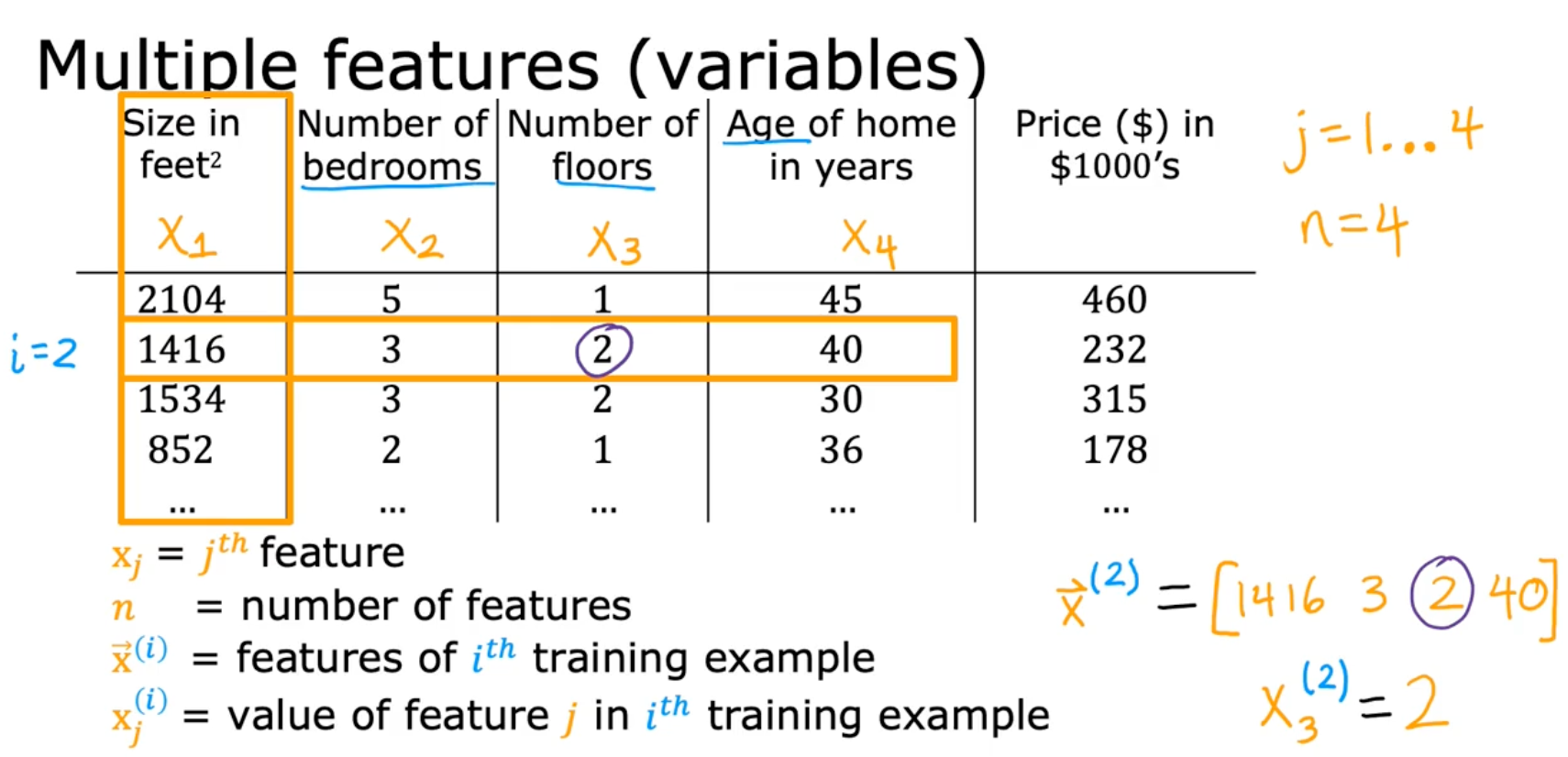
Multiple Features
Model
- parameters of the model
= [w1 w2 w3 .. wn]
- number
b
- vector
= [x1 x2 x3 .. xn]
Simplified - multiple linear regression
Vectorization
Parameters and features
= [w1 w2 w3] (n = 3)
b is a number
= [x1 x2 x3 .. xn]
w = np.array([1, 2, 3])
b = 4
x = np.array([10, 20, 30])
Without vectorization
f = w[0]*x[0] + w[1]*x[1] + w[2]*x[2] + b
f = 0
for j in range(n):
	f = f + w[j] * x[j]
f = f + b
With vectorization
f = np.dot(w,x) + bvectorization calculate each columns in parallel
- much less time
- efficient → scale to large dataset
Gradient descent
= (w1 w2 … w16)
= (d1 d2 … d16)
w = np.array([0.5, 1.3, ... , 3.4])
d = np.array([0.3, 0.2, ... , 0.4])
Compute for
Without vectorization
w1 = w1 - 0.1d1
…
w16 = w16 - 0.1d16
for j in range(16):
	w[j] = w[j] - 0.1 * d[j]
With vectorization
w = w - 0.1 * dGradient descent for multiple regression
Previous notation
Parameters
Model
Cost function
Gradient descent
repeat {
}
Vector notation
Parameters
Model
Cost function
Gradient descent
repeat {
}
Gradient Descent
One feature
repeat {
simultaneously update w, b
}
n features (n ≥ 2)
repeat {
j = 1 :
simulatenously update (for and
}
An alternative to gradient descent
Normal equation
- only for linear regression
- solve for w, b without iterations
- need to know
- Normal equation method may be used in machine learning libraries that implement linear regression
- Gradient descent is the recommended method for finding parameters w, b
- disadvantages
- doesn’t generalize to other learning algorithms
- slow when number of features is large (> 10,000)
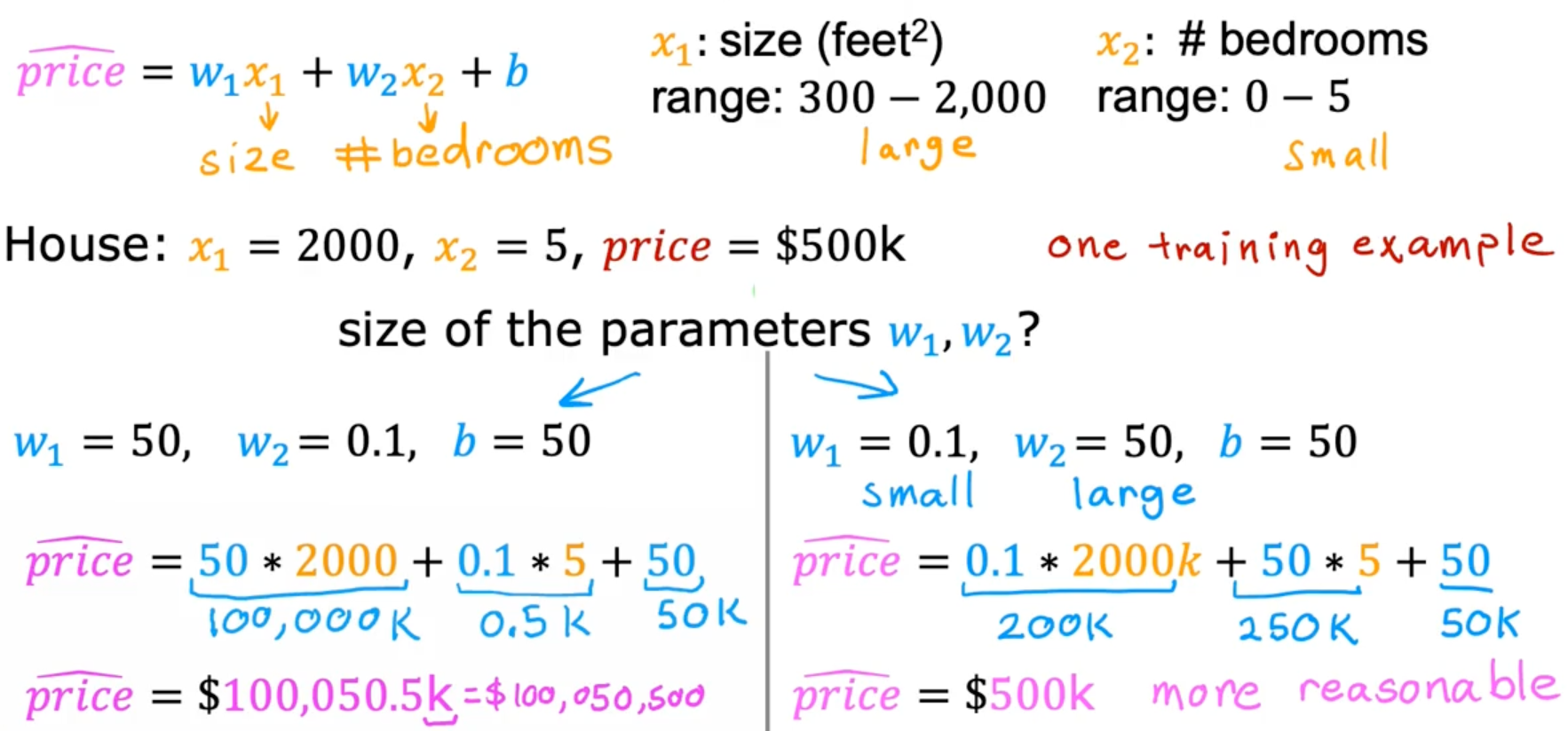
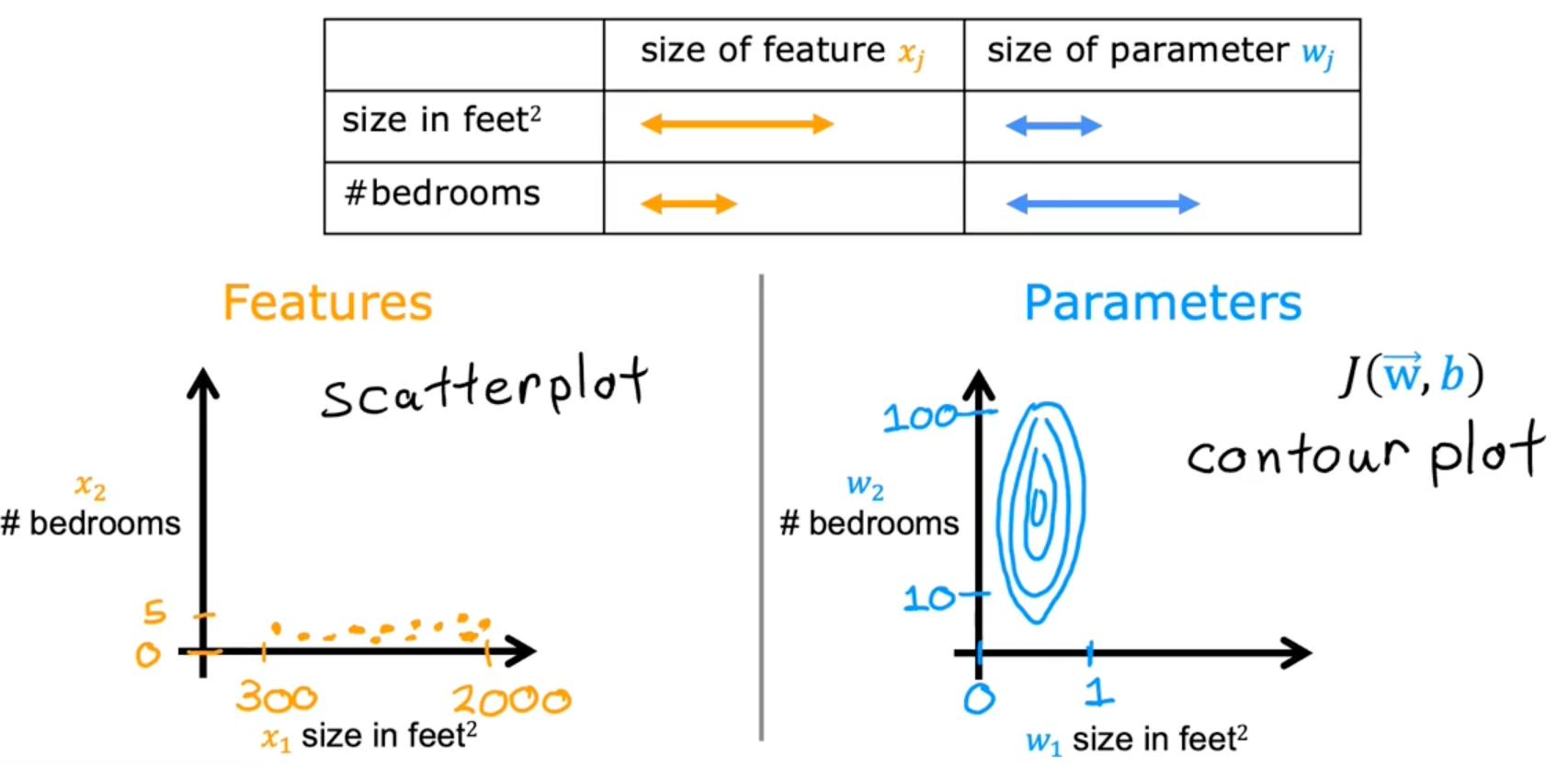
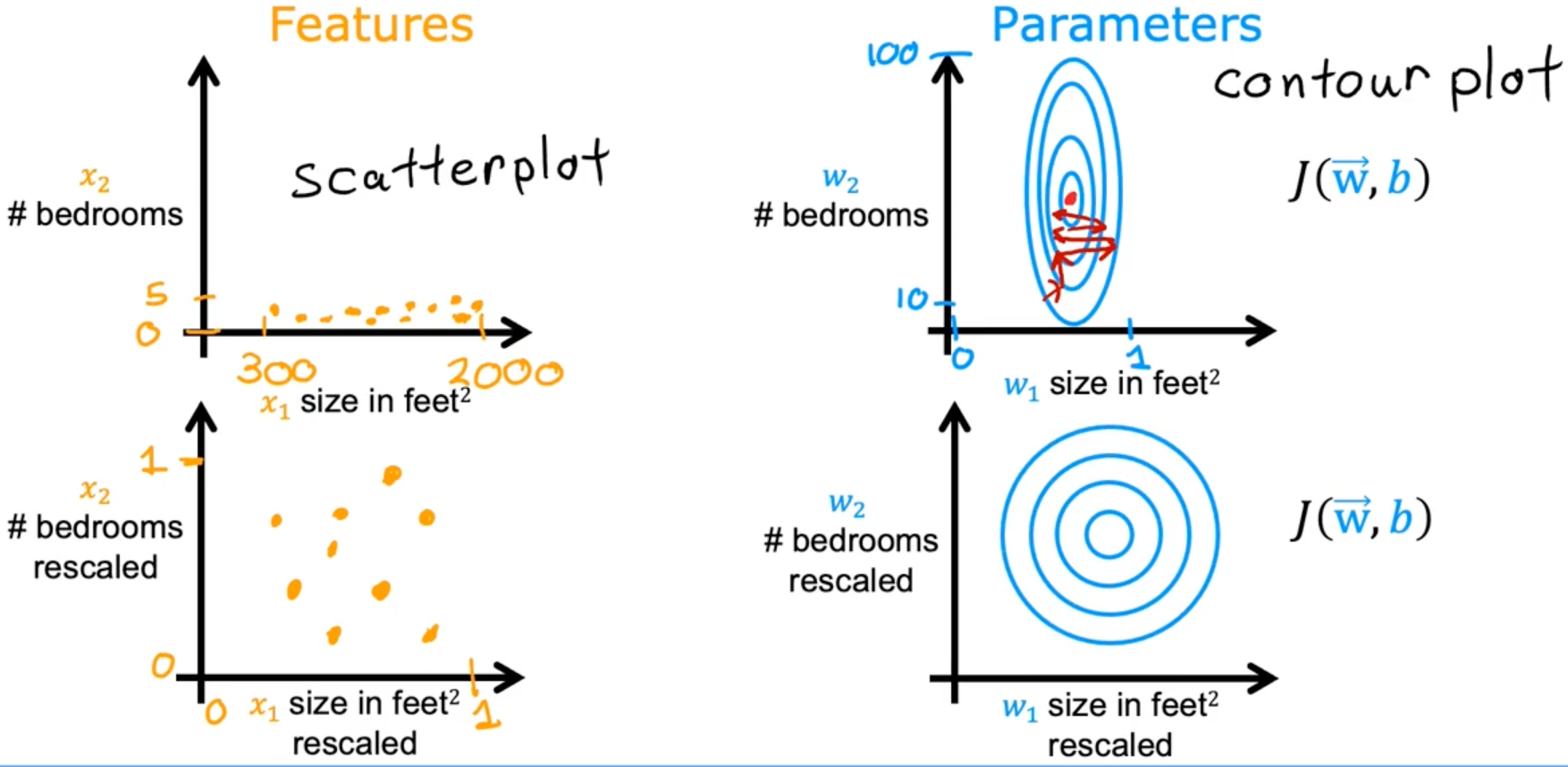
Feature scaling
Feature scaling enables gradient descent to run much faster by rescaling the range of each features
-
aim for about -1 ≤ ≤ 1 for each feature
- acceptable ranges
- -3 ≤ x ≤ 3
- -0.3 ≤ x ≤ 0.3
- Okay, no rescaling
- 0 ≤ x ≤ 3
- -2 ≤ x ≤ 0.5
- rescaling
- -100 ≤ x ≤ 100
- -0.001 ≤ x ≤ 0.001
- 98.6 ≤ x ≤ 105
- acceptable ranges
-
example
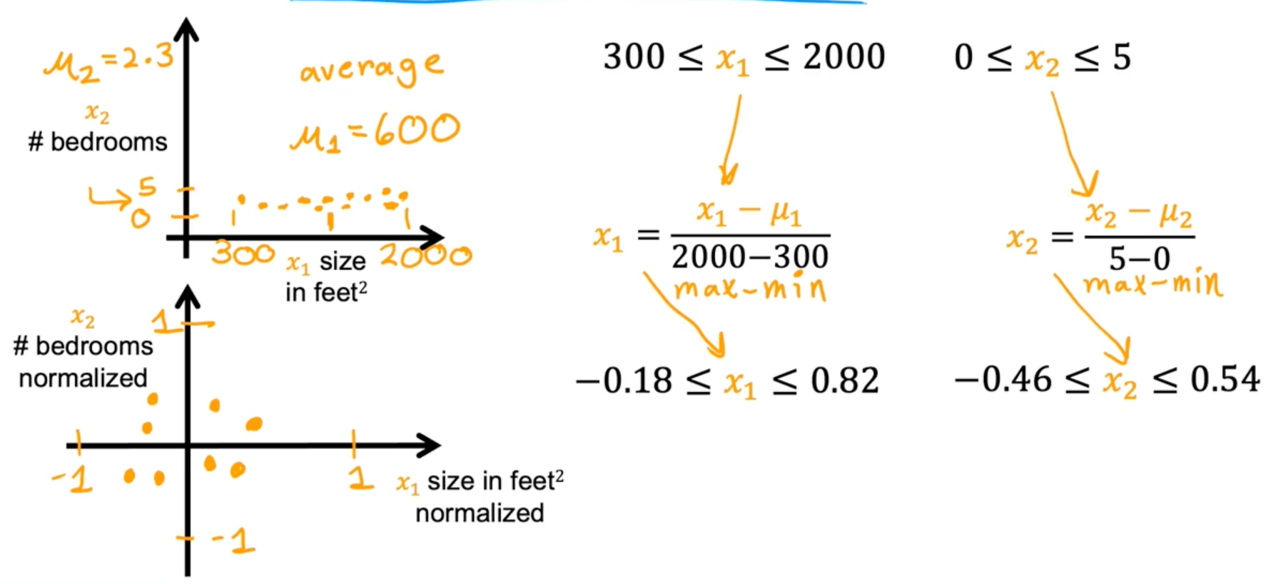
Mean normalization
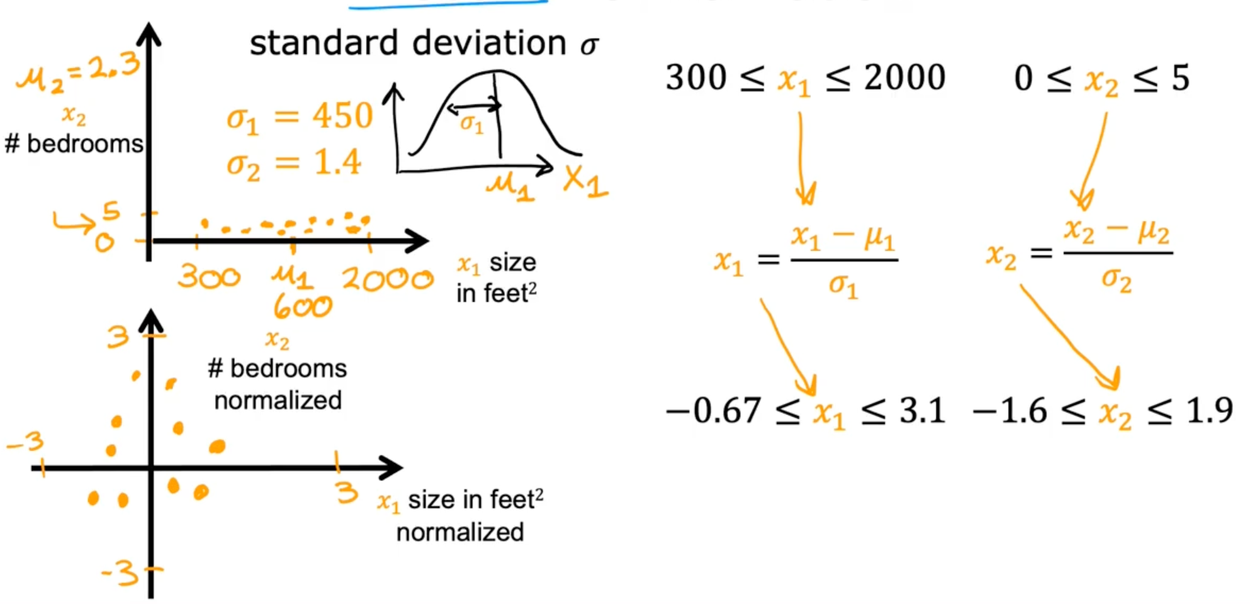
Z-score normalization
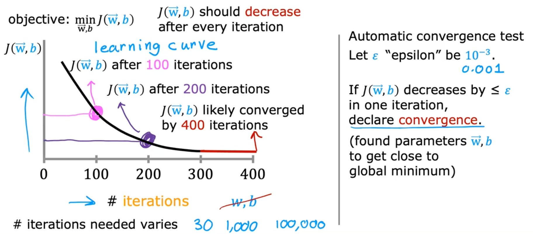
Checking Gradient descent for convergence
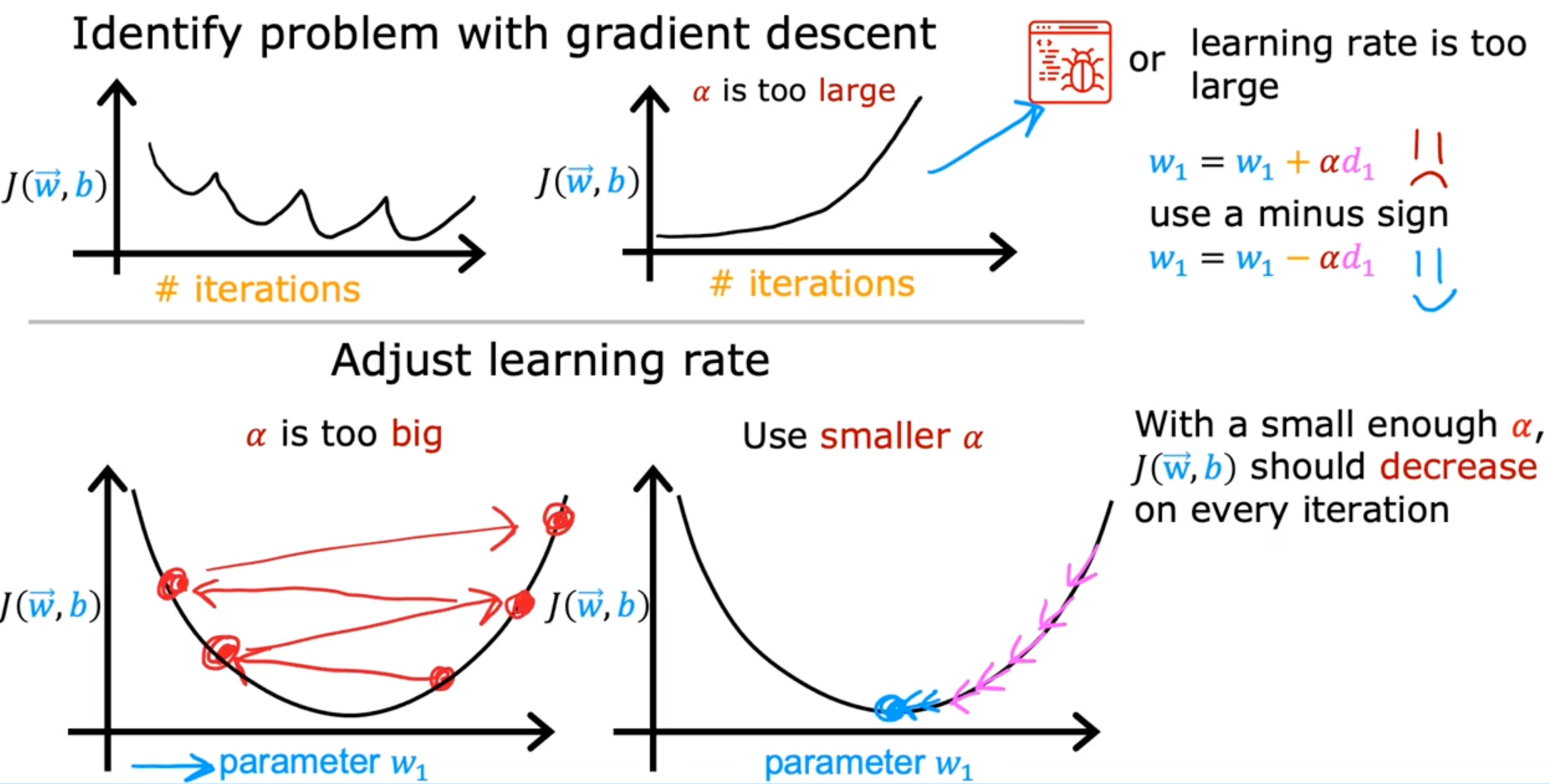
Choosing the learning rate
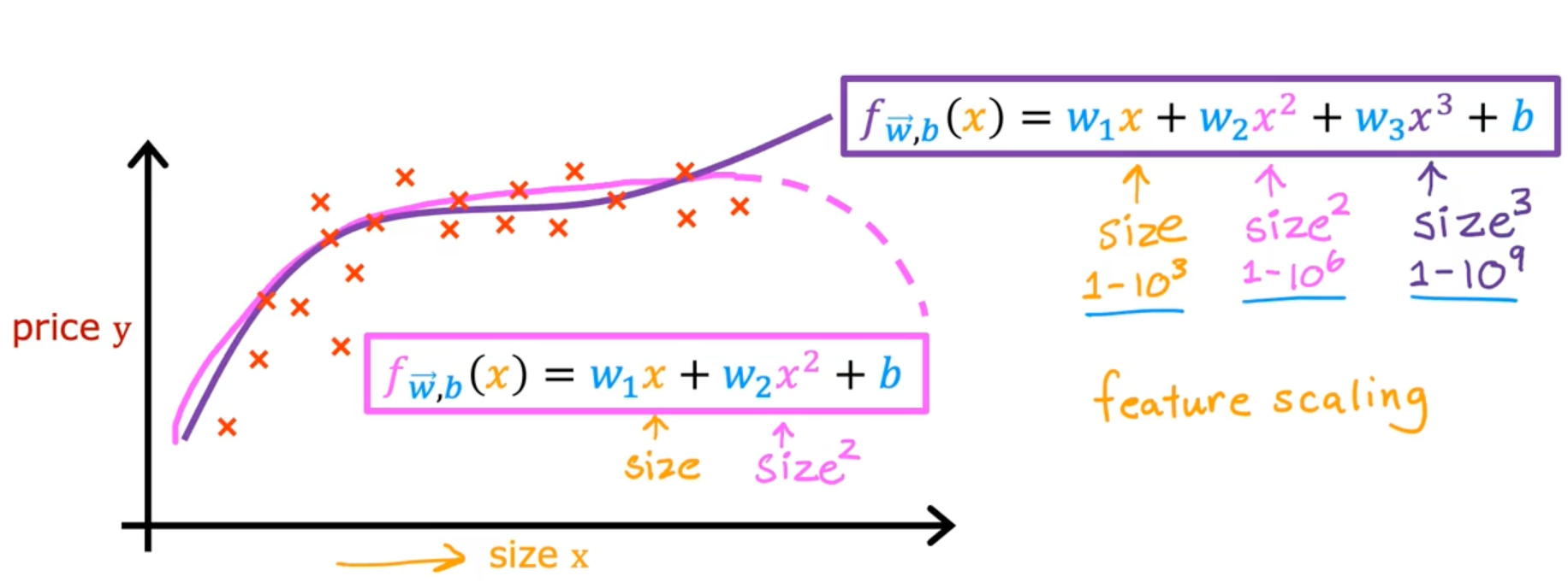
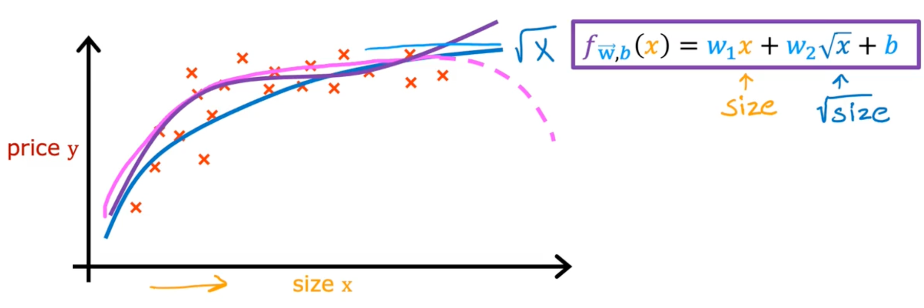
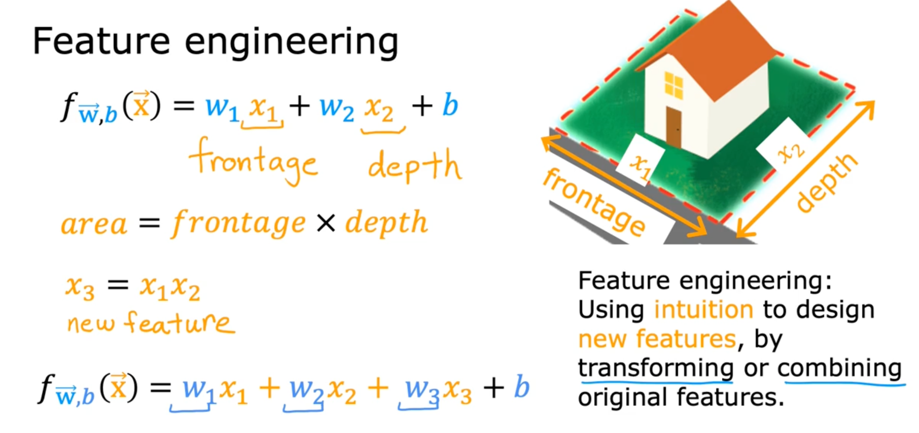
Feature engineering
Polynomial regression